Object ID: 00000018WIA30658870GYZ
Topic ID: id_40025091 Version: 1.2
Date: Apr 15, 2022 3:39:35 AM

Spectroscopy prescan

When a spectroscopy prescription is saved in the workflow manager, the Spectro Prescan button displays from the Scan menu.

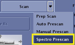
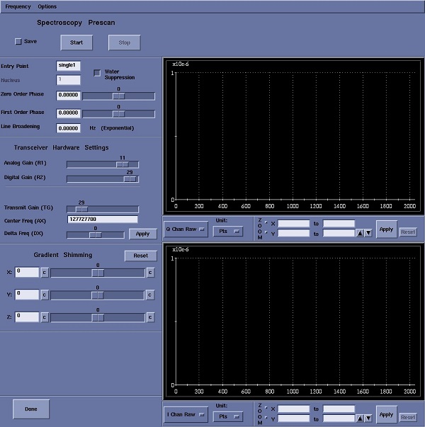
Click Spectro Prescan to open the Spectroscopy Prescan screen. This screen consists of two display windows, each with a display control panel just below the window, and a region at the left of the screen that allows for parameter entry, adjustment, and control.

APS is available for proton spectroscopy with all spectroscopy PSDs. When used in the image acquisition mode, the standard imaging APS entry points are executed to determine the receive and transmit gains (R1, R2, and TG), and the center frequency. In the spectrum acquisition mode, once the standard parameters have been determined, additional entry points may be executed to optimize the homogeneity, to optimize the water suppression, or to re-determine the transmit or the receive gains or the center frequency.

Note: A constant TR (1500 ms) is used during APS to prevent system time-outs or excessively long prescan times when long repetition times are prescribed.

There are nine integer values (0, 1, 2, 3, 4, 101, 103, 104 and 116) that correspond to eight APS entry points, and a Stop command. The integer values, the Entry Point names, and brief descriptions of the Entry Point functions are listed in the table below.

Figure 3. Entry point values, names and descriptions


Value	Entry Point Name	Entry Point Description
0	APS Stop Command	APS Stop value
1	CFL	Center frequency, low resolution
2	APS1	Sets TG, Same as Flip Angle TR
3	CFH	Center frequency, high resolution
4	APS2	Sets R1 and R2, Same as Scan TR
101	AWS	Automatic water suppression
103	AS	Autoshim, voxel localized
104	FASTTG	Fast TG determination
116	EXPRESS TG	eXpress TG determination

The APS process for each pulse sequence executes a predefined list of these entry points. The entry points in the list are executed in list order, and the list always ends with a zero, the APS Stop command.

The auto water suppression entry point (AWS, value 101) tries to find the optimum flip angle for the third presequence water suppression pulse. Voxel localized Autoshim (AS, value 103) uses the voxel size and center information from a pulse sequence to size and to center a shim volume around the prescribed voxel, the shim volume is slightly larger than the voxel. For the Fid CSI (MRS) and Echo CSI (MRS) slice selective sequences, the Autoshim process localizes according to the slice location(s) of the prescription. When Autoshim executes, data are acquired from three orthogonal slices centered on the voxel or slices, and used to determine the X, Y, and Z gradient current offsets

Display Waveform windows

There are two display waveform windows with control regions located immediately below each window. Each window has labeled horizontal and vertical axes: the numbers along the vertical axis represent the raw or processed signal intensity, and the numbers along the horizontal axis correspond to the selected unit label. The display control regions contain, from left to right, a display waveform pull-down menu, a pull-down menu to select a horizontal axis label, and horizontal and vertical zoom controls.

There are 14 waveform choices available on the display waveform menu; eight time domain waveforms and six frequency domain waveforms.

I Chan Raw: The real part of the complex raw signal is displayed.
Q Chan Raw: The imaginary part of the complex raw signal is displayed.
I - Q Chan Raw: The imaginary part of the complex raw data is subtracted, point-by-point, from the real part of the same complex raw data set. The result is displayed.
I^2 + Q^2 Chan: The square of the real part of a complex data point is added to the square of the imaginary part of the same complex data point for each complex data point in the signal. The result is displayed.
I^2 - Q^2 Chan: The square of the imaginary part of a complex data point is subtracted from the square of the real part of the same complex data point for each complex data point in the signal. The result is displayed.
I Filt: The real part of the raw complex data is multiplied, point-by-point, by an exponential filter (see Line Broadening in the section entitled Data Acquisition and Data Storage Commands below). The result is displayed.
Q Filt: The imaginary part of the raw complex data is multiplied, point-by-point, by an exponential filter (see Line Broadening in the section entitled Data Acquisition and Data Storage Commands below). The result is displayed.
Power: The real and imaginary parts of each complex data point in a processed data set (i.e., the raw data have been multiplied by an exponential filter and Fourier transformed) are squared and added. The resulting data set is displayed.
Magnitude: A magnitude spectrum is essentially the square root of a power spectrum. In this case, the square root of the sum of the squares of the real and imaginary parts of each complex point in the processed data set (i.e., the raw data have been multiplied by an exponential filter and Fourier transformed) is calculated. The result is displayed.
Uncor Real FFT: The real part of the uncorrected Fourier transformed complex data set is displayed. Uncorrected means that the raw data set was not multiplied by an exponential filter and that no phase corrections have been applied to the transformed data.
Uncor Img FFT: The imaginary part of the uncorrected Fourier transformed complex data set is displayed. Uncorrected means that the raw data set was not multiplied by an exponential filter and that no phase corrections have been applied to the transformed data.
Pure Absorp: The real (absorptive) part of a Fourier transformed complex data set is displayed. An exponential filter and phase corrections are applied to the data before they are displayed.
Pure Dispersion: The imaginary (dispersive) part of a Fourier transformed complex data set is displayed. An exponential filter and phase corrections are applied to the data before they are displayed.
Arctan2(Q/I): The arctangent of the point-by-point division of the imaginary part of the complex raw data by the corresponding real part of the complex raw data is calculated and displayed.
Unit: The units of the horizontal display axis. With time domain displays, the choices are msec (time in milliseconds) and Pts (points); for the frequency domain displays, the choices are Hz (Hertz), and Ppm (parts per million).
Zoom: The entries and selections in the zoom control area allow you to zoom along the horizontal (x) and vertical (y) axes.

Frequency

The Frequency selection allows you to save the current transmit frequency or to restore the transmit frequency that was previously saved. In common practice, neither of these options should be used. Saving a frequency other than a frequency in the proton chemical shift range may confuse the scan process.

Options

Click Options > Display Parameters to open the Display Parameters screen.

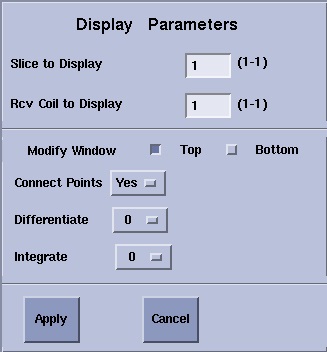
The current command settings are displayed on the panel. Changes to most of the parameters are only applied when you click Apply. The changes only apply to the top display, or to the bottom display depending on the current Modify window button selection (i.e., Top or Bottom).

Slice to Display is relevant for multi-slice acquisitions. A numeric range is displayed next to the text box. You can enter any integer value in that range. For example, if the range is (1 to 3), a signal is being acquired from each of three slices; to display the signal from the second slice, enter a 2.
Rcv Coil to Display is relevant for multi-coil data acquisitions. A numeric range is displayed next to the text box. You can enter any integer value in that range. For example, if the range is (1 to 3), a signal is being acquired from each of three coils; to display the signal from the second coil, enter a 2.
If the Connect Points selection is Yes, the points in the display are connected by a straight line; if it is No, the unconnected points are displayed. Changes are immediately applied to the data display.
Differentiate indicates the number of times that the data set is differentiated before it is displayed: 0, none; 1, once; and 2, twice.
Integrate indicates the number of times that the data set is integrated before it is displayed: 0, none; 1, once; 2, twice; and 3, thrice.

Data Acquisition and Data Storage commands

Figure 7. Data acquisition and storage screen area

Data acquisition is controlled with the Start and Stop buttons. The Save button saves raw data to the computer disk.

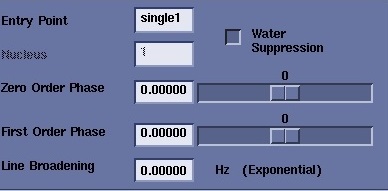
The Start button starts the acquisition of raw spectral data using the scan prescription that you entered on the Scan Desktop, with the exception of using the data acquisition mode specified by the Entry Point selection, typically single1 or avg. With the default single1 Entry Point selection, data are continuously acquired and displayed until Stop is clicked. Depending on the value of NEX, a single excitation (NEX = 1), or an average of several excitations (= NEX, where NEX is 2 or more), is acquired, displayed, and then overwritten by the next excitation(s). With the single1 entry point, you can use the Zero Order Phase and First Order Phase sliders and/or the text boxes to correct the phase of a Pure Absorption display. It is often desirable to smooth or to enhance the resolution of a spectroscopy data set by multiplying the raw data with a windowing or filter function. The filter function is an exponential of the width specified by the entry (in Hz) in the Line Broadening text box. A copy of the raw data is multiplied by the exponential filter prior to the Fourier transform. The default Line Broadening value is zero (0.0).

If the Entry Point is changed to avg, clicking Start initiates the collection of a signal averaged data set where the number of excitations corresponding to the total number of scans User CV is combined into a single data frame. As the data are collected, they are displayed in the display windows on the Spectroscopy Screen. Data collection and data display updates terminate automatically when the selected number of excitations (equal to the total number of scans) has been acquired. When acquiring data with the avg Entry Point, it is not possible to change the zero and first order phase settings, or the line broadening value. For most pulse sequences, data acquisition with the avg Entry Point is very similar to the acquisition of a data set using the Scan button on the Scan Desktop; the major difference is that with avg, all excitations are combined to create a single data frame.

Click Save to write the raw data acquired on the Spectroscopy screen to the /usr/g/mrraw directory on the host computer. The Save button may only be clicked after an acquisition has been terminated either automatically or with the Stop button. Raw data must be saved before a subsequent acquisition is started, since the raw data buffers used by the Spectroscopy screen processes are always overwritten when Start is clicked.

Transceiver Hardware Settings

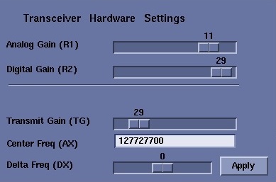
The sliders and type-in entry fields in the Transceiver Hardware Setting area provides access to the transceiver hardware settings – center frequency, and transmit and receive gains – that are normally determined and set by the Auto Prescan process or on the Manual Prescan screen.

Analog Gain (R1): is the true receive gain. A change of one unit corresponds to a change of 3 dB in the receive gain. The allowed range of R1 is 1-13.
Digital Gain (R2): corresponds to the number of digital bits used by the receiver during data acquisition and digitalization, and, ultimately, to the number of bits in each data word. Allowed values are 1-30 with the selection of the Extended Dynamic Range Imaging Option. The range is 1 to 15 if the EDR option is not selected. With the EDR option selected, each data word occupies 32 bits of memory (two sign bits and 30 data bits), without EDR each word occupies 16 bits of memory.
Transmit Gain (TG): can be adjusted in a range from 0 to 200, where each unit corresponds to a 0.1 dB change in the transmit gain.
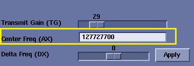
Center Freq (AX): allows you to enter an explicit entry of the RF center frequency in Hertz. The initial center frequency value that appears depends on which nucleus is chosen during the acquisition prescription. The nucleus value is determined automatically from the connected coil. The selected mass number is displayed (but can not be changed) on the Spectroscopy Screen in the panel just above the Transceiver Hardware Settings panel as the Nucleus value. A default center frequency is calculated from the current setting of the center frequency – typically that of hydrogen – using a ratio of the current gamma to the selected gamma. Occasionally the gamma ratio may yield an unacceptable center frequency and generate a warning or an error message.
Delta Freq (DX): allows you to select and apply a small frequency change (in Hertz) to the frequency that appears in the Center Freq (AX) field.

Gradient Shimming

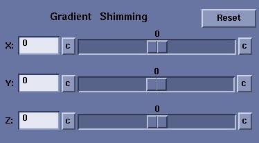
The Gradient Shimming area allows you to adjust the linear (x, y, and z) shims by adjusting the corresponding gradient currents. Sliders for each gradient current can be adjusted in a small range around the current settings or you can enter gradient current offset values in the X, Y, and Z text boxes.

Click c at either end of the sliders to re-center the range around the current gradient current offset setting.
Click Reset to restore the initial current offset values at any time.
The X, Y, and Z gradient labels correspond to the physical (i.e., the actual) gradient axes, which may differ from the logical gradient axis labels used in the pulse sequences.

Adjusting the homogeneity through manual shimming is neither fast nor easy, particularly for nuclei other than hydrogen. The hydrogen based Autoshim capability is both fast and reliable, and should be used to optimize the shim whenever possible. In all voxel localized hydrogen spectroscopy, Autoshim should be selected to optimize the shim through the voxel during the APS process. Generally, Autoshim should always be selected during the acquisition of a localizer image that corresponds to the slice or plane from which the spectrum will be acquired. It is often worthwhile to run Autoshim as part of the APS process for the exact slice of the spectroscopy prescription, and/or to use Autoshim in the APS process of a voxel localized sequence to optimize the shim in a specific region in a slice.

Message window

The Spectroscopy screen message window is the unlabeled region just below the Gradient Shimming panel. Status messages, such as Spectro Acquisition has started, are displayed in this window.

Done

Click Done to leave the Spectroscopy screen. Clicking Done during an ongoing data acquisition terminates the acquisition. The unsaved raw data are lost, but the current Spectroscopy screen parameter settings are retained.