
- 00000018WIA30978970GYZ
- id_400263511.4
- Mar 28, 2022 3:58:38 PM
fMRI
Functional imaging or BOLD provides fMRI analysis using the Correlation Coefficient algorithm to analyze an image set. Neuronal activity of either motor or cognitive functions can be mapped by fMRI through changes in signal intensity arising from bulk magnetic susceptibility-induced relaxation changes resulting from variations in blood flow and oxygenation. A common technique to detect activation in an fMRI study is cross correlation. With this approach, activated pixels are those identified as having a high correlation with a reference function (pattern) that characterizes activation-induced signal change. The resulting functional maps can be used for mapping the motor cortex and higher cognitive regions of the brain.
fMRI imaging is typically used in surgical planning to identify areas of eloquent brain. It is also used for cognitive studies, psychiatric evaluation, and treatment monitoring.
A fMRI image acquisition sequence is typically a single shot, multiphase, GRE-EPI sequence with a limited number of slice locations and a high number of phases. During the acquisition, a task (simulation) is performed in an on and off or active and rest state. Task activation or stimulation of an area of the brain increases the oxygen level, which increases the T2* weighting and the resulting signal intensity. The type of task/stimulation used is driven by the area of interest in the brain. The reference pattern is determined by the TR. Use the following formula to calculate the paradigm time:
- TR (in seconds) x reference pattern = paradigm time
- 3000 TR × 10 = 30 second paradigm time
- 2500 TR × 10 = 25 second paradigm time
In the example of a 3000 TR with a 30 second paradigm, 10 phases at each location are collected when the patient is not performing the task, then 10 phases at each location are collected when the patient is performing the task. This pattern is repeated until 128 phases are collected at each location (the last group will only have 8 phases at each location).
GRE-EPI produces a brighter “flash” image than SE-EPI, but the extra CNR from the GRE-EPI makes it preferable as the pulse sequence. Using a 60° rather than a 90° flip angle can decrease the brightness from the flash image, but it will compromise SNR. Therefore, typically use a 90° flip angle.
Algorithms
Correlation Coefficient
The algorithm returns a value, on a pixel-by-pixel basis, that characterizes similarity between the temporal variations in time course data and a user-specified reference pattern.
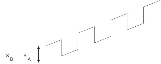
The time course data sets are correlated with a generic reference pattern that is a periodic “boxcar” function of the form:
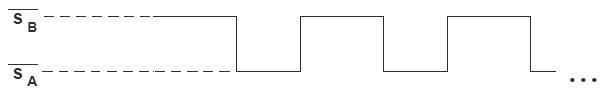
The boxcar function oscillates between two signal levels sA and sB.
The correlation coefficient cc of the time course data to this reference function is related to the Student’s t-test parameter (t) by the following relationship:
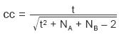
where the Student’s t-test parameter (t) is a value that characterizes the difference between the two mean values, sAand sB, of the time course data. The mean value sA is determined from a subset (A) of the time course values and the mean value sB is determined from an independent subset (B) of the time course values. The subset (A) are those time course values that coincide with the reference function in its “A” state and the subset (B) are those that coincide with the reference function in its “B” state.
The generic definition of the Student’s t-test parameter is given by:

where  is the standard error, defined as:
However, since actual time course data may include baseline drift, the data will be correlated with a boxcar function with a linear drift or slope added of the form:
In order to properly calculate the difference, the time course data will be fitted to a linearly sloped boxcar function using linear regression analysis. The three-parameter linear regression analysis will return the values for , the slope of the linear drift, and the initial value of
  . The linear regression analysis will also return a value equivalent to the standard error, , described above.
From these results, the t parameter will be calculated and, subsequently, the correlation coefficient, cc.
The confidence level of the correlation coefficient parameter will be defined as:
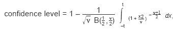
where t is the Student’s t parameter, v is the “degrees of freedom” given by:
v = NA + NB –1
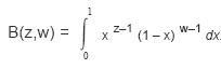
and B is the beta function given by
Confidence levels defined in this way have small values corresponding to high “confidence” and large values corresponding to low “confidence.” For example, a confidence level of 0.001 indicates a 0.1% probability that the time course data are not correlated to the reference function.
The user-defined confidence level is used to threshold the correlation coefficient calculation such that:
- Thresholded cc = cc if confidence level </= user-defined confidence level
- 0 if confidence level > user-defined confidence level
The pixel locations for which the algorithm returns 0 are displayed in black on the functional map.
The algorithm generates functional maps for the correlation coefficient as described above, and for the activation magnitude, defined as the amplitude of the boxcar function fitted to the time course data.
The active state of the activation function can induce either an increase or a decrease of the signal; hence, the correlation coefficient and activation magnitude at a given pixel location can also be either positive or negative. The positive and negative correlation coefficient and activation magnitude are displayed in separate functional maps.
When this algorithm has been selected, the drift-adjusted boxcar function fitted to the time course data is also shown on the graph view, either as a blue curve for the cursor ROI curve or as a red curve for the currently selected user ROI.
Input parameters
Reference pattern: this is defined by the user by means of three parameters:
- NS: the number of images to skip at the start of the exam
- NA: the number of images in the active state
- NB: the number of images in the inactive state
This allows the user to ”synchronize” the exam data with the activation pattern used at acquisition.
Confidence level: by default a confidence level of 0.1% (0.001) is used, but this value can be changed from the protocol.
fMRI measurement units
The fMRI functional maps have the following units of measurement.
| Maps | Units |
|---|---|
| Positive Activation magnitude | N/A |
| Positive Correlation magnitude | N/A |
| Negative Activation magnitude | N/A |
| Negative Correlation magnitude | N/A |
READY View protocols that use fMRI scan data
fMRI