

- 00000018WIA30EFF870GYZ
- id_400241451.6
- May 26, 2022 9:51:59 AM
PROBE 2D CSI: acquire a scan
Before you begin
About this task
In order to display the localizer image in READY View, the center of each reference slice must be within 0.8 mm of each CSI slice. If a slice that meets this criterion does not exist in the selected reference series, READY View displays an error message, "Localizer loading failed, no matching image". Click OK to the error message. READY View launches, but an image does not display in the lower-left viewport. To avoid this problem, follow these guidelines when prescribing a 2D CSI scan.
Important: Do not save the 2D CSI protocol as an oblique plane. Save the protocol as an axial plane and then change the plane to oblique when you are viewing/editing the series.
Step-by-step instructions
- To change the VOI shape, click Grid from the Graphic Rx Spectro menu and only change the VOI shape on the image that displays the CSI Grid.
Figure 1. Example of: Axial image displaying CSI grid 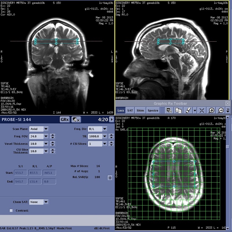
- Verify that the VOI is bisected by the yellow reference line in the two planes that are orthogonal to the plane in which you deposited the VOI.
- In the following example, the VOI was deposited on the axial image. In image A the VOI size was only adjusted on the axial image. The VOI is bisected by the yellow lines in both the sagittal and coronal images. In image B, the VOI size was changed by clicking and dragging the VOI in the coronal plane. When the reference lines are displayed, it is clear that the VOI is not bisected by the yellow lines in the coronal and sagittal planes. The results are the following:
- Image A will display the localizer when READY View is launched.
Figure 2. Image A. Note that the VOI is bisected by the yellow cross reference lines 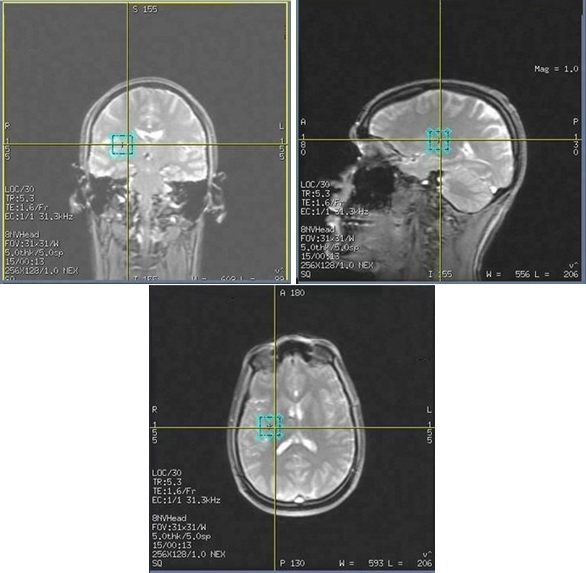
- Image B will NOT display the localizer when READY View is launched.
Figure 3. Image B. Note that the VOI is off center from the yellow cross reference lines. This prescription will NOT launch the localizer in READY View 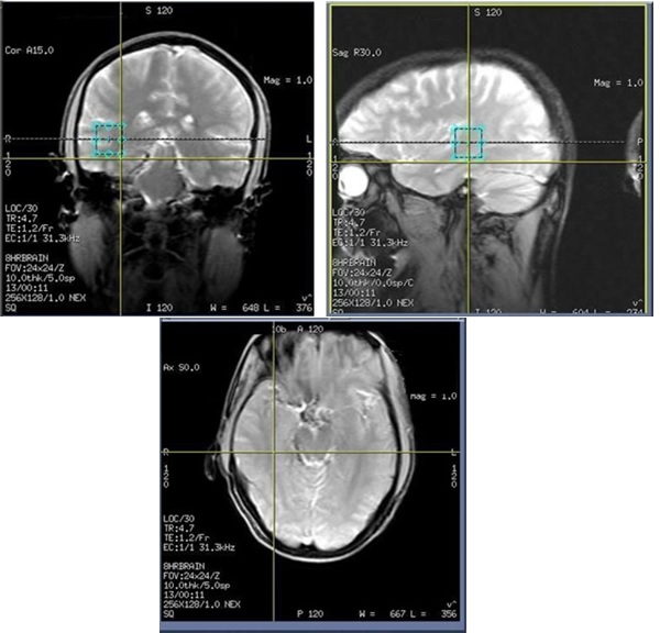
- Image A will display the localizer when READY View is launched.
- In the following example, the VOI was deposited on the axial image. In image A the VOI size was only adjusted on the axial image. The VOI is bisected by the yellow lines in both the sagittal and coronal images. In image B, the VOI size was changed by clicking and dragging the VOI in the coronal plane. When the reference lines are displayed, it is clear that the VOI is not bisected by the yellow lines in the coronal and sagittal planes. The results are the following: